A geographic approach to housing price prediction

🛒 Introduction

Initial meetings with real estate clients often involve a reality check around price expectations. A buyer may assume they can get far more for their money than the market supports; a seller may expect a price well above what comparable homes are fetching. Either way, misaligned expectations make deals harder to close.

Predicting house prices from features is a classic machine learning problem — and neighborhood is almost always a key factor. But neighborhoods are rarely defined consistently: some span many blocks, others just a few. What if, instead of assigning each house a categorical neighborhood label, we estimated its geographic value as a continuous feature? Could that improve prediction accuracy? This project explores housing sales data from Ames, IA using several machine learning models, and deploys the results in an interactive R Shiny dashboard.

🖥️ Exploratory Data Analysis

Visualization of the neighborhoods

As explored in New York City: Booms and Blooms, neighborhoods develop through successive waves of construction. The first map below shows house age across Ames: Old Town is the oldest, with newer neighborhoods radiating outward toward the town perimeter.

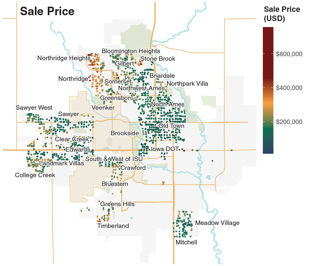
The second map shows sale prices. Most homes that sold above $400,000 are in the newer outer neighborhoods. Northridge Heights and Northridge stand out — their median sale prices were more than 2× the citywide median of ~$160,000.

Most homes in Ames are single-family houses, with a median sale price of around $160,000 from 2006–2010. Price scales strongly with living area, as shown by the regression line below.

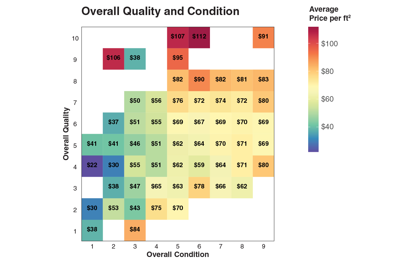
Dividing price by area gives price per ft², which normalizes for size. The two strongest predictors of price per ft² are overall quality and condition — higher-rated homes command a clear premium.

👨‍🔧 Feature Engineering

Neighborhood labels in this dataset are inconsistent, and some neighborhoods have fewer than ten sales — too few to avoid overfitting. Rather than using a categorical neighborhood feature, we engineered a continuous geographic value score derived from the trained model. This score captures how much a location adds to a home's price, independent of the home's physical features.

A house with identical features will be worth more in a high-geographic-value area. Interestingly, geographic value correlated inversely with local crime rate — areas with more crime had lower geographic values.

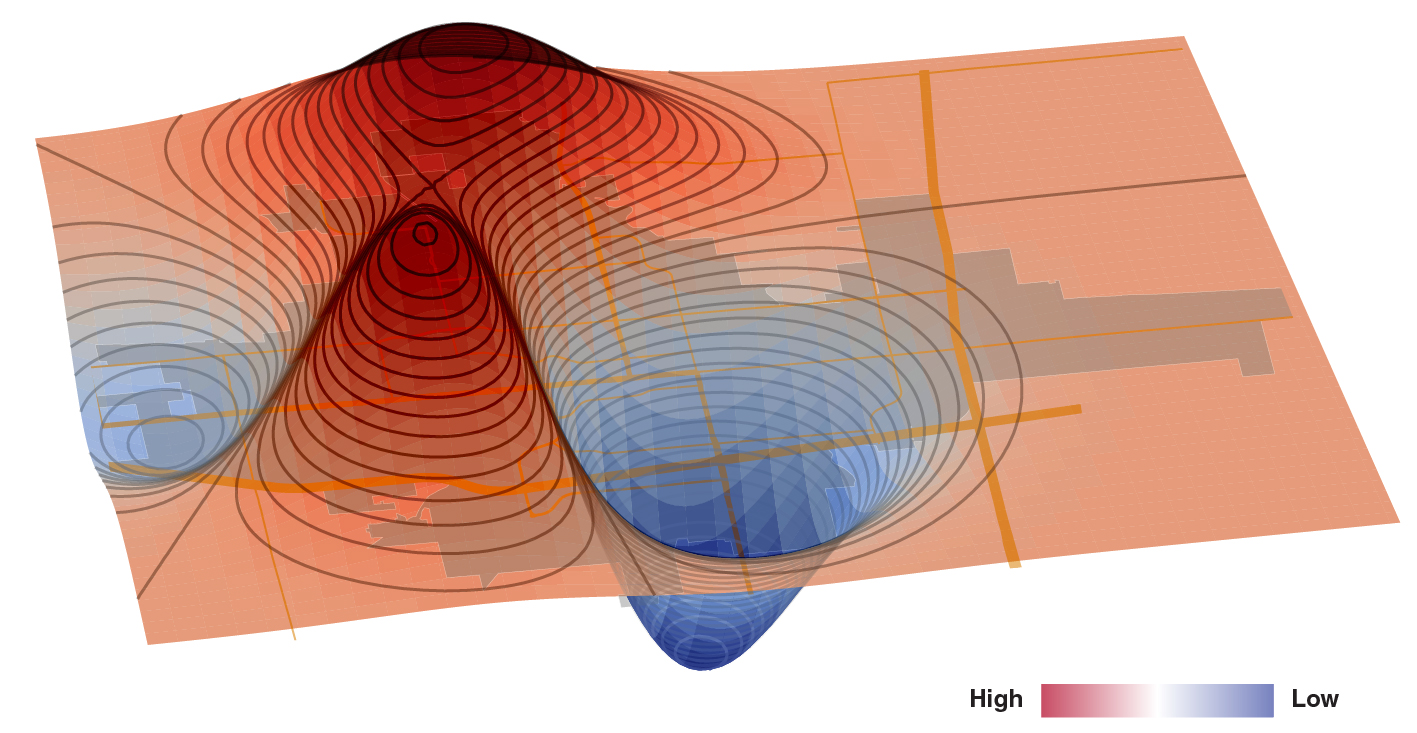
The 3D surface below maps geographic value as height. The prominent peak at the front corresponds to the Iowa State University campus area — a notable hotspot, as Ames is a college town.

🦾 Machine Learning Models

Starting from 145 features (including one-hot encoded and engineered variables), EDA reduced the set to 45, and Lasso Regression further narrowed it to 32. Data was split 70/30 into train and test sets.

Lasso and Ridge Regression

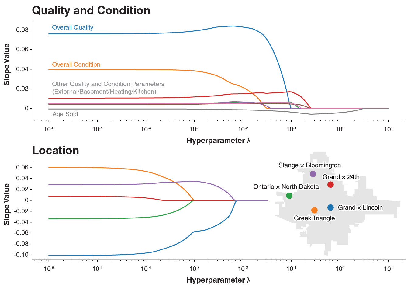
Lasso Regression was used first to eliminate low-signal features. The plot below shows how coefficients shrink as the regularization parameter λ increases (log scale) — features that persist to high λ have the most predictive power. Quality and condition are the strongest survivors.

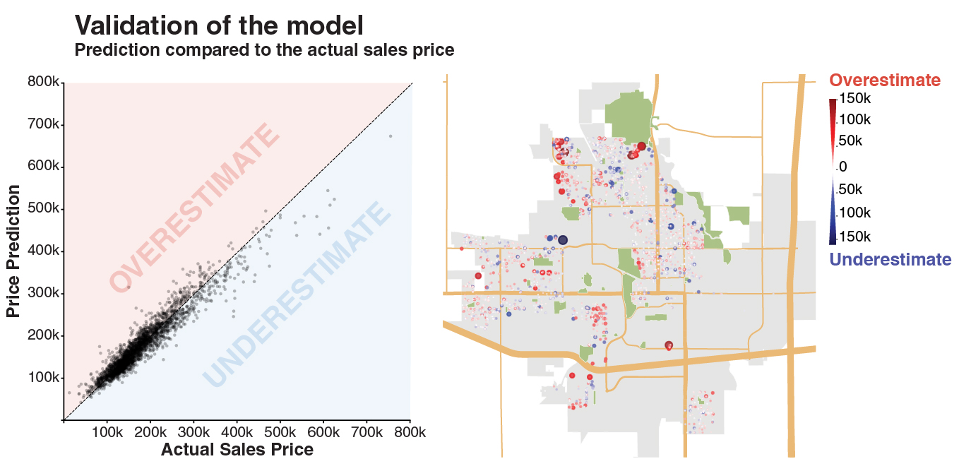
Ridge Regression with cross-validated λ = 0.0032 achieved R² = 0.900. The plots below compare predicted vs. actual prices, and a residual map highlights where the model over- (red) and under-predicts (blue).

Other ML Methods

Additional models were tested with grid-searched hyperparameters. Results are summarized below.

Method	Best R²	Hyperparameters
Lasso Regression	0.900	CV = 3 λ = 10⁻⁵ Normalized
Ridge Regression	0.900	CV = 3 λ = 0.0032 Normalized
SVR	0.918	RBF kernel ε = 0.1 γ = 0.01
Random Forest	0.899	500 trees 7 max features subsample = 0.8 col sample = 0.8
Boosting	0.922	5000 trees 7 max features learning rate = 0.01
XGBoost	0.923	5000 trees 7 max features learning rate = 0.01 γ = 0.01 subsample = 0.8 col sample = 0.8

📱 Shiny App

Best viewed on large screens

📝 Conclusion

Square footage, overall quality, and condition are consistently the strongest predictors of house price.
ML models achieved R² scores of 0.90–0.92 on held-out test data.
A continuous geographic value feature — derived from model residuals — outperforms categorical neighborhood labels and correlates with local crime rates.
XGBoost achieved the best performance (R² = 0.923), with ensembles generally outperforming linear models.
The results are deployed in an interactive R Shiny app for exploration and price prediction.

This project was developed by Chad Loh, James Reno, Michelle Bui, and Alex Galczak.

Data Source

Ames Housing dataset — compiled by Dean De Cock for data science education